Learn how you can Unlock Limitless Customer Lifetime Value with CleverTap’s All-in-One Customer Engagement Platform.

In the previous article, we discussed what an outlier is and ways to detect such outliers with parametric and non-parametric methods by conducting a univariate and bivariate analysis. Let’s now look at Clustering, a non-parametric method and a popular data mining technique to detect such outliers when we are dealing with many variables or in a multivariate scenario.
Clustering groups set of objects in such a way that objects or observations in the same group or cluster are more similar to each other, than those in other groups or clusters. The important term here is ‘similar’. Somehow, we need to quantify ‘similar’ in the context of clustering. This could be quantified with a distance measure. Different Clustering techniques employ different distance measures to arrive at the goal of forming clusters; we shall concentrate on K-means clustering, a popular and most widely used clustering technique.
K-means clustering is implicitly based on pairwise Euclidean distances. Euclidean distance is the “ordinary” (i.e. straight-line) distance between two points. There are other distance metrics like Manhattan, Minkowski, Chebychev distance apart from Euclidean distance that can be used but K-means may stop converging with other distance functions.
Given a set of observations (x1, x2, …, xn), where each observation is a d-dimensional real vector, k-means clustering aims to partition the n observations into k(≤ n) sets (S = {S1, S2, …, Sk}) so as to minimize the within-cluster sum of squares (wss) (sum of distances of each point in the cluster to the Kth center). In other words, its objective is to find: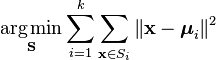
where μi is the mean of points in Si.
The above formula will become clear as we discuss the basic steps in K-means clustering and the evaluation metric for identifying the right number of clusters with it.
Step 1: Deciding the Number of Clusters
Select the number of clusters or segments. There is no magic formula to calculate this before hand and it has to be an iterative process. We will discuss ways and means to evaluate it with an example.
Step 2: Assigning Centroids
Randomly select the number of observations or points, which are equal to the number of clusters. So if we have decided on having 5 segments, randomly select 5 observations from your dataset and assign them as Centroids.
Step 3: Distance from Centroids
Calculate the distance of each of the observation from the centroids and assign the points to the closest centroid. For example: In a dataset of 100 observations, you would calculate the distance of each of those observations from the centroids. For a particular observation and 5 centroids, you will end up with 5 distances. The observation gets assigned/grouped to the cluster containing the centroid from which it has recorded the lowest distance.
Step 4: Recalculate Centroids
The center point or the centroid of the clusters is recalculated. The centroid is like the mean of the observations/points and is calculated in the same way as you calculate the average or the mean of points. So, if the points in the cluster change due to assignment of the observations to different clusters in Step 3, the mean or the centroid of that cluster could change.
Step 5: Repeat
Repeat Step 3 and Step 4 until the Centroids don’t move.

One important point to bear in mind before running the K-means algorithm is to standardize the variables. For example, if your dataset consists of variables like age, height, weight, revenue, etc which are essentially incomparable, it will be a good idea to bring them on the same scale. Even if variables are of the same units but with quite different variances it is better to standardize before running the K-means algorithm. K-means clustering is “isotropic” in all directions of space and therefore, tends to produce more or less round (rather than elongated) clusters. In this situation, leaving variances unequal is equivalent to putting more weight on variables with smaller variance, so clusters will tend to be separated along variables with greater variance. Standardization will ensure that K-means gives equal weightage to all the variables. A quick way to standardize a variable is to take the difference of each observation from the mean of the variable and divide such difference by the standard deviation of the variable.
Now let’s use K-means to identify outliers. This is possible assuming you have the right number of clusters and one of the clusters, due to its characteristics is totally or substantially different from other clusters. This will become clear with an example given below: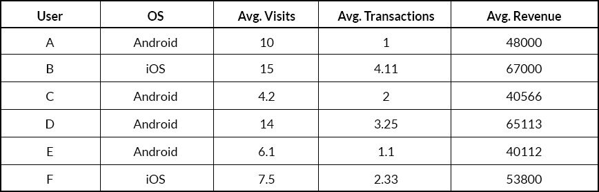 The above table is a subset of the user data of an app. We have 5 columns/variables with 3 numerical variables and 2 categorical variables. We will ignore Column 1 for our analysis.
Use of Categorical Variables in K-means
We could convert the categorical variable (‘OS’) to numerical by encoding Android as ‘0’ and iOS as ‘1’ or vice-versa. But, conceptually it is not advisable to do so and run a K-means algorithm on it due to the manner in which K-means calculates the distance in the Euclidean space. Can you quantify distance between a Android and iOS as 1 or 2 or any other number just as we can easily quantify the distance between 2 numerical points ?
For example: if the Euclidean distance between numeric points A and B is 30 and A and C is 8, we know A is closer to C than B. Categorical values are not numbers but are enumerations such as ‘banana’, ‘apple’ and ‘oranges’. Euclidean distance cannot be used to compute distances between the above fruits. We cannot say apple is closer to orange or banana because Euclidean distance is not meant to handle such information. For this reason, we won’t be including the categorical variable in the K-means algorithm. For categorical variables, a variation of K-means known as K-modes, introduced in this paper by Zhexue Huang, could be suitable.
Estimating Number of Clusters
Getting the right number of clusters is an iterative process. To get the right number of clusters, we shall try running the K-means with 2 to 20 clusters for the above example and look at some common evaluation metric to arrive at that number. As an analyst, running the iterative process over higher or lower number of clusters is your prerogative. But, before running the K-means algorithm, we will standardize the numerical variables to bring them on the same scale.
To evaluate the ideal cluster size, there are various metrics like within sum of squares, between sum of squares, percentage of variance explained by the clusters, gap statistic, etc. For the above example, we shall track the within sum of squares.
Within sum of squares (wss):
This metric essentially gives us the homogeneity within a group. The metric calculates the sum of squares of the distance of each point in a particular cluster from its respective centroid. We shall refer to it as ‘wss’. You will calculate ‘wss’ for each of the cluster. The sum total of wss for all the clusters is the Total wss (twss).
The metrics mentioned above are relative and not absolute metrics i.e. their values have to be compared with the number of clusters chosen. The metric for a particular cluster number, say 2, in the above case, can’t be viewed in isolation. It has to be compared with all the clusters ranging from 3 to 20. If we have to choose between 2 and 20 as the ideal number of clusters, we will tend to go with the cluster number that has the lowest twss in the above case.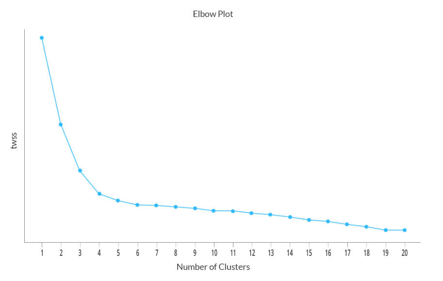
The above graph plots the total within sum of squares (twss) for number of clusters between 1 and 20. From the graph, it seems that the rate of change for twss decreases substantially after 4 clusters. Theoretically, you would tend to choose the lowest twss, but practically it might not be the best option. As per the graph, it seems that the right number of clusters is 19 but analyzing such a large number of cluster tends to be tedious and may not achieve the required goal as the distance between many clusters may not be significant and could be close to each other. In this example, we see that there is a steep decline in twss until 4 clusters, after which the rate of change decreases rapidly. Hence, we shall go with 4 as the number of clusters. You might even consider analyzing with different cluster sizes and compare the cluster characteristics between all such chosen clusters before arriving at the best cluster size.
Visualizing Clusters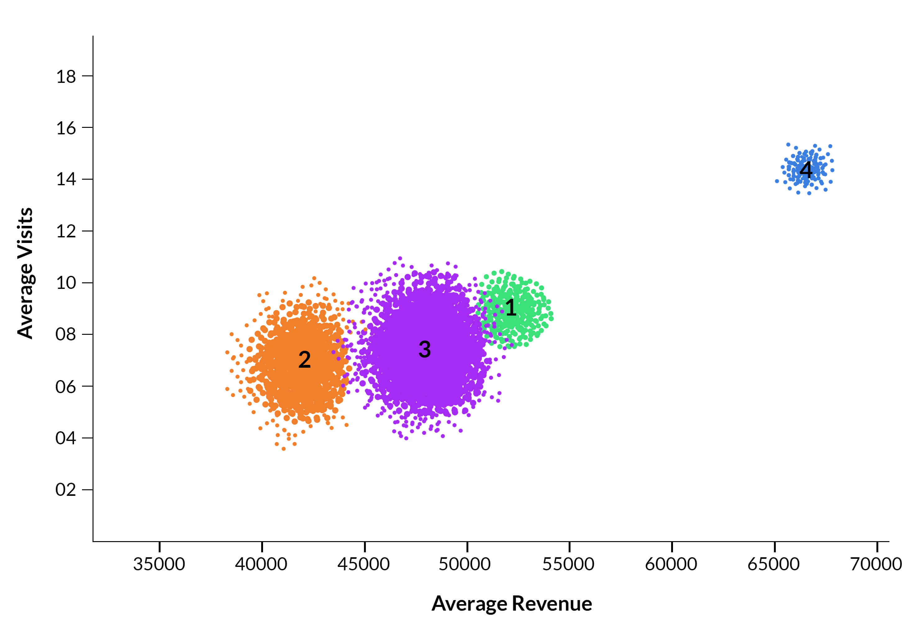
The different colors for the points indicate their membership for different clusters. There is one cluster i.e. Cluster 4 that is very different or far from the other clusters, the points for which are in colored in ‘blue’.
Cluster Characteristics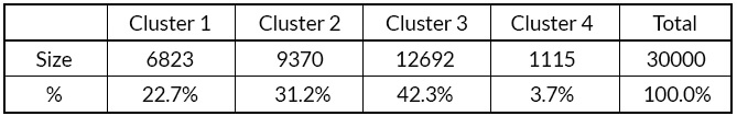
The above table gives the size or the number of observations in each cluster. Cluster 4 has 3.7% of the observations and is the smallest of the lot.
Let’s look at some more characteristics of the clusters formed.
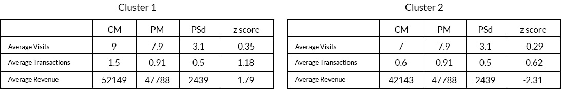
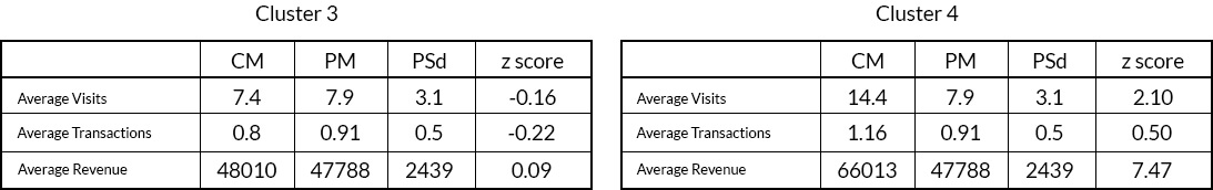 CM – Cluster Mean ; PM – Population Mean ; PSd – Population Standard Deviation
The above table shows the mean of the variables observed in the cluster and compares it to the overall mean observed for those variables and uses a Z-score to quantify the distance between the cluster and the overall mean.}{\sigma }}")
where: μ is the mean of the population and σ is the standard deviation of the population.
For each numerical variable, the Z-score, basically, normalizes the distance of the cluster mean from the overall mean by dividing such distance with its standard deviation. For the same mean difference, the variable that has a lower standard deviation will have a higher Z-score between the 2 variables. The sign of the Z-score indicates whether the group mean has been above or below the overall mean.
Cluster 4 seems to stand out in the above table considering factors such as lower number of observations, higher number of visits, transactions, average transaction value, and high Z-scores.
Let’s also take a quick look at the cluster characteristics in terms of OS, the categorical variable.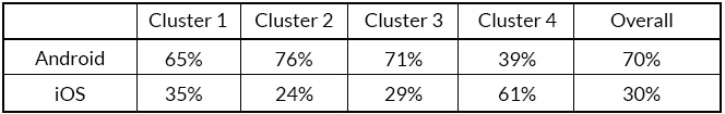
The proportion of iOS users in Cluster 4 is significantly different from all the other clusters. Thus, it could be concluded based on the above evidences that Cluster 4 is an outlier and observations in it could be considered as outlier candidates. As an analyst, one should delve deeper into Cluster 4 to understand the key factors driving the behavior of the users in this cluster since its users have not only interacted more with the app but also spent more compared to users in other clusters.
In conclusion, we have been able to identify outliers in a multivariate scenario with the help of clustering, a non-parametric approach. There are a number of clustering algorithms apart from K-means that one can experiment to identify such outliers, based on the characteristics of the dataset, but is beyond the scope of this article.