Learn how you can Unlock Limitless Customer Lifetime Value with CleverTap’s All-in-One Customer Engagement Platform.

Being a sci-fi movie buff, I would always wonder if my variables could turn into Autobots just like the movie ‘Transformers’ and make my life building statistical models that much easier. Until that day, I will have to use the available tools to transform my variables.
Data Analysis
Before drawing valuable insights or building predictive models, an analyst will try to probe deeper and understand the data thoroughly. We often go about analyzing the variables present in the dataset by visualizing them one at a time i.e. univariate analysis before proceeding towards analyzing 2 or more variables jointly i.e. multivariate analysis. Histograms are often the default choice of visualizing numerical continuous variables.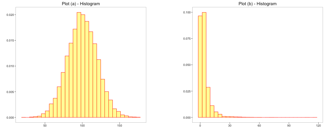
The above charts depicts histograms of 2 different variables. Breaking the numerical variable into intervals formed the histograms and the bars indicate the area occupied by the number of observations in that particular interval. The spread of the bars in the 2 histograms are different indicating how the observations are distributed along the intervals. It helps us view the symmetry of the data i.e. the upside mirrored by the downside? When you look at the shape, you are trying to make certain inferences about the distribution of variables.
Why does distribution matter?
Distribution helps you identify the likelihood or probability of an observation or an interval. For example: you could infer in (a) above, majority of the data is between values 50 to 150 whereas, in (b), it is between 0 and 20 even though the range of the data is much higher. Depending on the shape of the distribution, you would tend to estimate the likely chance of observing a value or range of values. The choice of averages like mean, median and mode also tend to depend on the type and shape of the distribution.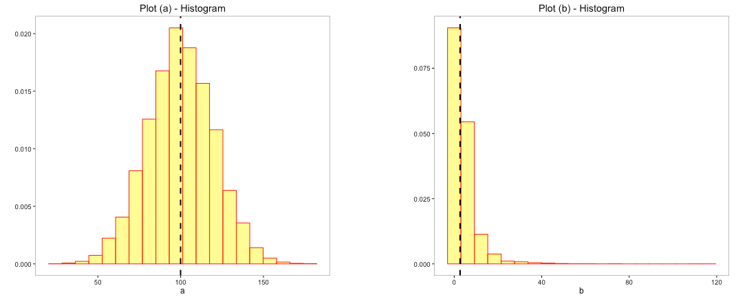
The dashed line indicates the chosen average for the variables. While mean could be a good average for the plot (a), median could be a good average for plot (b).
Type of Distribution
Plot (a) above closely resembles a Normal distribution. The shape of the normal distribution resembles a bell and it is symmetric around the mean. Normal Distribution is an extremely important distribution in the field of statistics as many statistical tests and models require that the data is normally distributed. In practice, we work with data that is close to a normal distribution. Normal distribution assumes that the numerical data is continuous.
Transformation of Non-Normal Data
Data in the real world is often non-normal. Since normality of data is one of the key assumptions of many statistical tests, transformation of non-normal data to normal data or near normal becomes important. Here, we are dealing with transforming numerical continuous data.
For example: Suppose you have a variable ‘y’ and are tasked with exploring the relationship with ‘x’.
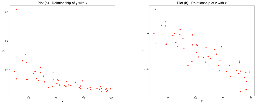
Plot (b) clearly depicts a stronger linear relationship between the variables compared to plot (a). The variable ‘y’ in plot (a) was transformed to the new variable ‘z’ which reflected a distribution that is close to normal distribution. Plot (b) used the transformed variable ‘z’ and the resultant plot showed a stronger linear relationship.
Let’s discuss some of the ways to convert non-normal to normal with the task of converting 5 different numerical variables given below: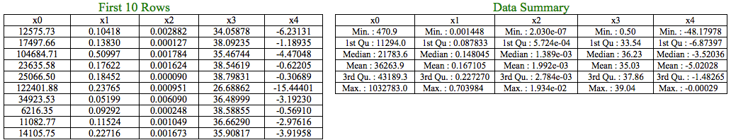
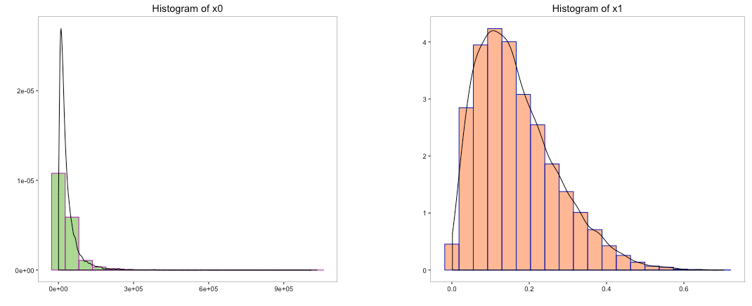
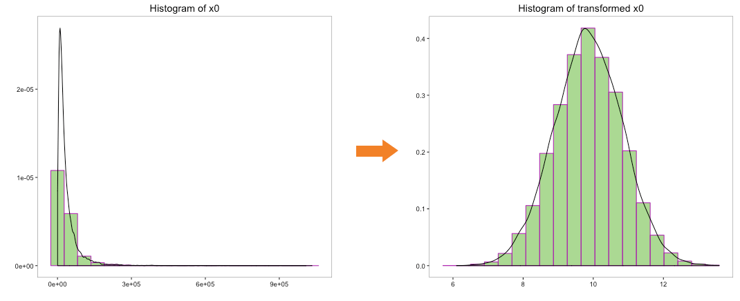
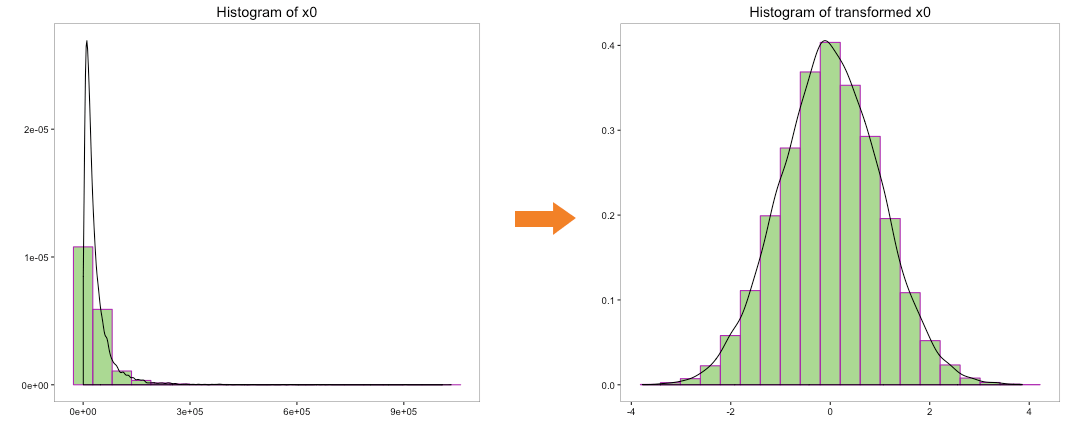
Let’s begin with plot (a) and try to convert its distribution to normal distribution. Many a times, taking the log of a dataset does the trick.
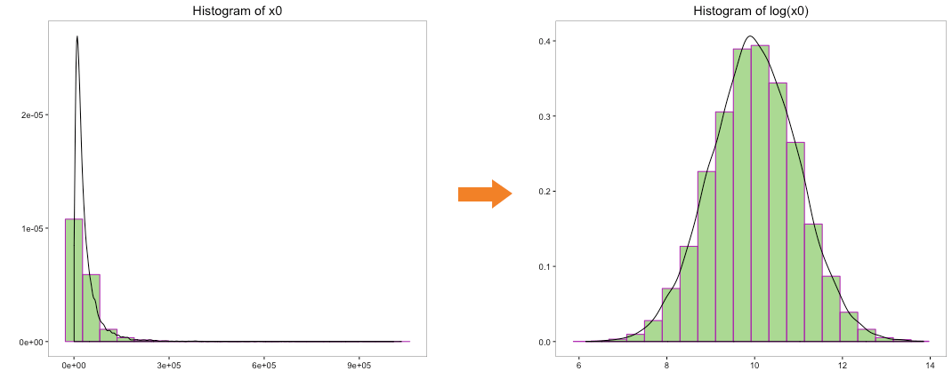
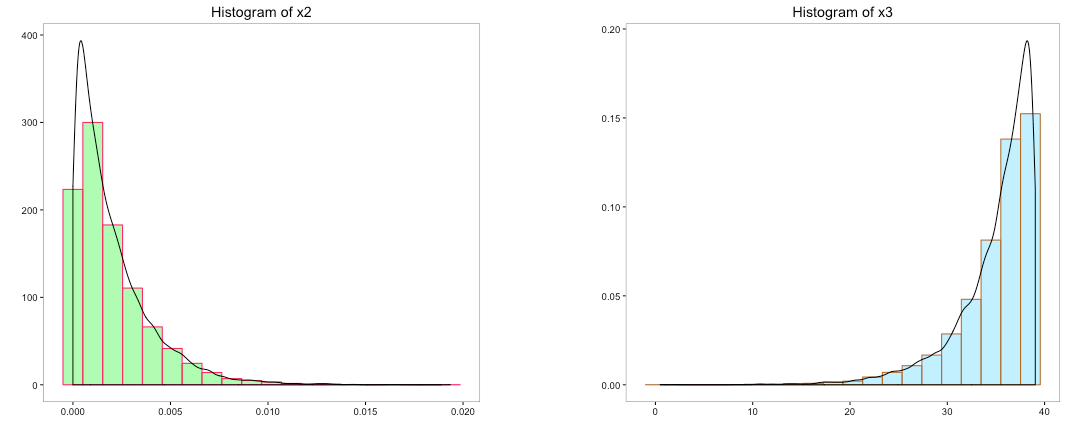
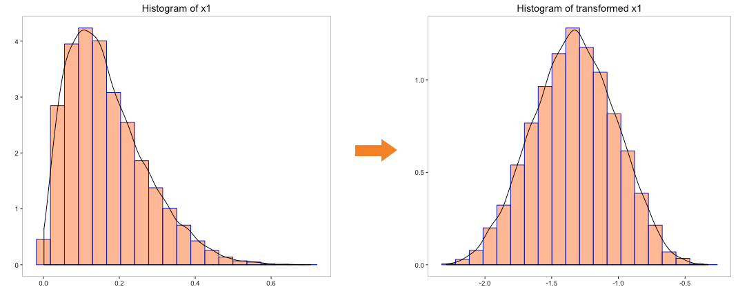
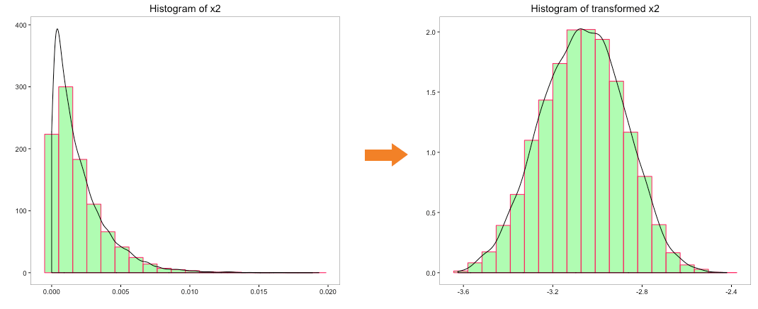
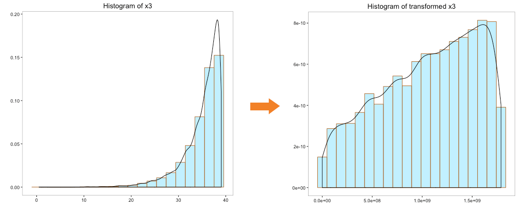
The above histogram does indicate that the distribution of ‘x0’ is transformed to normal distribution. But can we use log to convert the other variables as well. We cannot take the log of a negative number so variable ‘x4’ can be ignored. Let’s take the log of the variables ‘x1’, ‘x2’ & ‘x3’ and view their histograms:
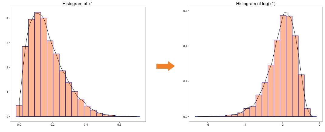
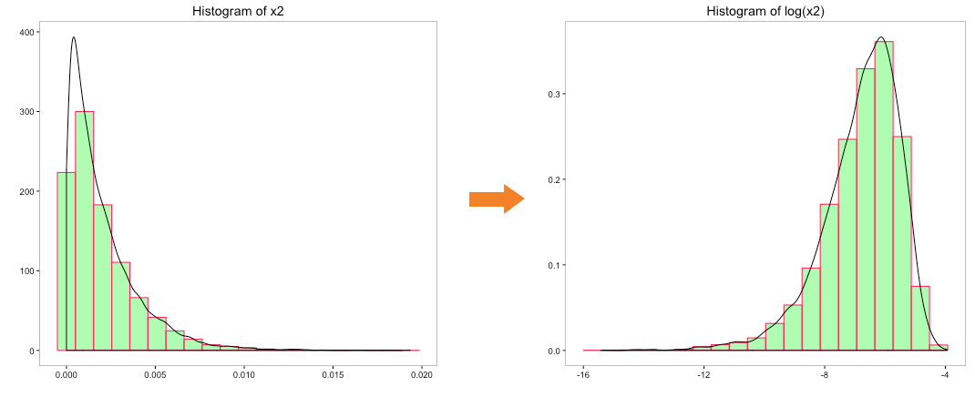
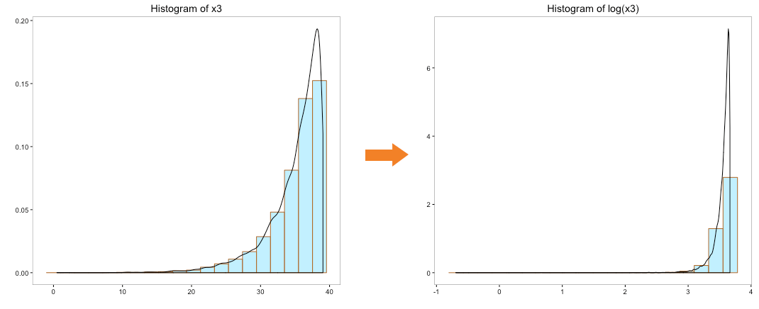
Though transformation of ‘x1’ and ‘x2’ does hold some promise, transformation of ‘x3’ is clearly not acceptable. We could use some of the other tricks such as taking the square, square root, cube root, etc. of the variables. All these tricks can be quite tedious to execute as it involves trial and error method with no guarantee of transformation to normality.
What-if we could programmatically generate a parameter, which could then be used to transform the data to reflect normal distribution. We will discuss 2 such methods, Box-Cox and Johnson transformation to achieve our objective.
Statisticians George Box and David Cox developed a procedure to identify an appropriate exponent (Lambda = λ) to use to transform data into a “normal shape.”

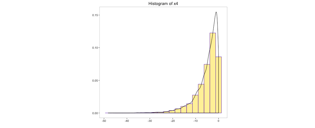
The Lambda value indicates the power to which all data should be raised to transform it to normal. In order to do this, the Box-Cox power transformation searches from Lambda = -5 to Lambda = +5 until the best value is found. Box-Cox like log transformation works with non-negative numbers. One can always transform the variable to reflect only non-negative numbers but we won’t be able to anticipate new incoming data and perhaps, the data may still contain negative numbers. Hence, we would not consider transformation of ‘x4’.
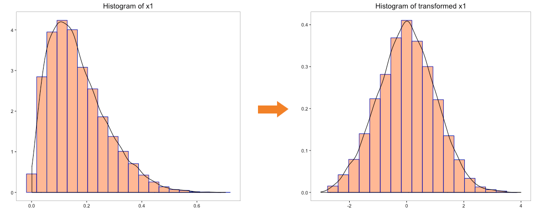
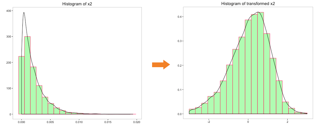
Let’s try to convert the distribution of the variables ‘x0’, ‘x1’, ‘x2’ and ‘x3’ to normal distribution using box-cox transformation:
The distribution of transformed variables ‘x0’, ‘x1’ & ‘x2’ using box-cox looks better than the log transformation and quite indicative of a normal distribution. Transformation of ‘x3’ doesn’t indicate a normal distribution.
Johnson Transformations is considered to be more powerful since it can also work with negative data unlike Box-Cox transformations.
For Johnson transformations, one needs to estimate the parameters as given by the evaluation of 3 functions given below:
Bounded system (SB):
Log-normal system (SL):
Unbounded system (SU):
where:
; y = transformed value; γ = shape 1 parameter; η = shape 2 parameter; ε = location parameter; λ = scale parameter.
One needs to evaluate all three functions with the estimates of all the parameters in the formula, transform the data and run normality test on the transformed data. All the parameters are optimized until one of the three transformation functions produces the best normality test result. Thankfully, like box-cox, we don’t need to manually do the heavy-lifting work as most statistical software tools typically do this.
Let’s run the Johnson transformation on variables ‘x0’, ‘x1’, ‘x2’, ‘x3’ and ‘x4’ and look at the histogram post transformation:
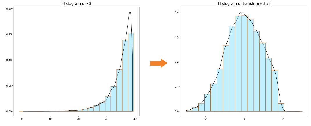
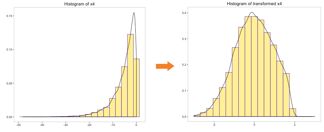
The above histograms indicate that underlying distribution of the transformed variables is closer to normal. More importantly, Johnson transformation has been able to transform the distribution of variable ‘x4’, which has negative numbers.
The Trial & Error method to transform variables could result in the loss of productive time of an analyst since the probability of parameter identification to transform the non-normal distribution is similar to the probability of winning a lottery. Hence, choosing between the Trial & Error method and Programmatic method is quite easy and the preferred choice for an analyst ought to be the Programmatic method. But, the trickier question would be the choice within the Programmatic method i.e. between Box-Cox and Johnson transformation. The choice between the methods could boil down to 2 key considerations:
Box-Cox transformations won’t work with negative numbers whereas there is no such restriction for Johnson transformations. You can precede the transformation by adding a constant number to all the observations, thereby converting the negative numbers to non-negative. However, it would be extremely difficult to anticipate any new observation to be non-negative even after adding the earlier assumed constant to it. Hence, a better choice is Johnson Transformation, in case of the variables that contain or could contain negative numbers.
The computational cost of transforming variables using Johnson transformation is much higher than Box-Cox transformation due to presence of higher number of parameters that needs to be optimized. Hence, you are better off with Box-Cox transformation, if the objective is to minimize computational cost of transforming the variables.
In case of transformation of non-negative numbers, an alternative approach could be to use both Box-Cox and Johnson transformation and then select the method, which transforms the variable distribution closer to normal.
Life is not perfect, so is the dataset that an analyst works with. In this article, we learnt how we could use Box-Cox and Johnson transformations to convert the non-normal distribution of variables to near normal distribution and make it palatable to statistical modeling. Though, the methods mentioned are extremely useful, one needs to apply them with caution and rigorously test the normality of the transformed variables with more than just histograms. Suitable tests like Anderson-Darling test and visualization techniques such as Q-Q plot to check for normality should be used.
Box-Cox and Johnson Transformations could prove to be your own neighborhood Autobots but beware; their indiscriminate use could just turn them into Deceptions. Nevertheless, the above 2 techniques should be a part of the arsenal of an astute statistical analyst.
Check out this R code that shows how to use box-cox and johnson transformation with the help of a simple example.