Learn how you can Unlock Limitless Customer Lifetime Value with CleverTap’s All-in-One Customer Engagement Platform.
In the real world, we often come across scenarios which requires to make decisions that result into finite outcomes, like the below examples,
All the above situations do reflect the input-output relationships. Here the output variable values are discrete & finite rather than continuous & infinite values like in Linear Regression. How could we model and analyze such data?
We could try to frame a rule which helps in guessing the outcome from the input variables. This is called a classification problem, and is an important topic in statistics and machine learning. Classification, a task of assigning objects to one of the several predefined categories, is a pervasive problem that encompasses many diverse applications in a broad array of domains. Some examples of Classification Tasks are listed below:
Mostly, in the business world, Classification problems where the response or dependent variable have discrete and finite outcomes, are more prevalent than the Regression problems where the response variable is continuous and have infinite values. Logistic Regression is one of the most common algorithm used for modeling classification problems.
Why do we need Logistic Regression?
In case of Linear Regression Model, the predicted outcome of the dependent variable will always be a real value which could range from –ꝏ to +ꝏ. But unlike Regression problems, in Classification problems, the outcome value is either 0 or 1 or any other discrete value, as we saw in the above listed common examples. Now the question that arises is how to ensure that we only get the predicted outcome value as 0 or 1 after fitting a linear model for Classification problems.
To answer this question, let’s consider a couple of cases involving two variables:
Case I: Y is a linear function of X say $ \ y = Bx $
Case II: P is a non-linear function, say, an exponential function of R i.e. mathematically expressed as
$ P = e^{R} \ or \ P = exp\left ( R \right ) $
While Y is a linear function of X, can we instead make some transformation to express P as some linear function of R? The appropriate transformation that could be applied in Case II is “Log” transformation.
Applying log on both sides of Case II equation, we get = \textup{R} \textit{ i.e. } log\left ( P \right ) \emph{is a linear function of 'R'}")
Let’s leverage our understanding of Linear Regression Analysis, by using some trick – like some transformation to solve Case II scenarios, to develop methodology for solving Classification type of Problems.
So, what’s Logistic Regression?
Logistic Regression is a type of predictive model to describe the data and to explain the relationship between the dependent variable (having 2 or more finite outcomes) and a set of categorical and/or continuous explanatory / independent variables.
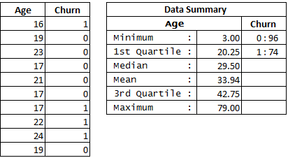
Suppose you have a dataset of 170 users containing the user’s age and whether or not the user tend to churn out from an app. The goal is to predict the tendency of the user to churn for a particular user’s age. The subset of 10 rows of this dataset and its summary is displayed below:
The above dataset can be visualized graphically as below: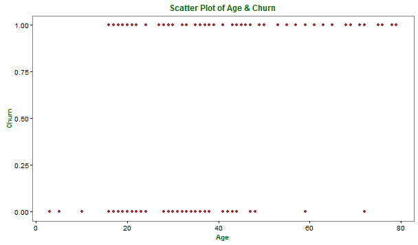
It appears in the above graph that the target outcome variable, Churn, has a value 1 if the user is active / not churned on the app and 0 if the user churns out from the app.
Can we simply use Linear Regression to describe this relationship?
Let’s try to determine the best fit line by applying linear regression model, which is depicted in the following plot: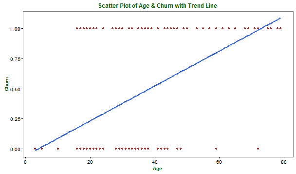
Upon inspecting the above graph, you notice that some things do not make sense as mentioned below:
Such values are not possible with our outcome variable (Churn) as they fall outside its legitimate and meaningful range of 0 to 1, inclusive. That implies, the line does a poor job of “describing” this kind of data.
Then the question arises: How to overcome these problems of Linear regression model? Is it possible to then model churn by some other technique?
Since Linear Regression requires variables to be measured on continuous scale, let’s recode Age into a new categorical variable AgeGroup of 6 categories. Then, we compute the Churn percentage (Non-churning users of an AgeGroup / Total users count for an AgeGroup) for each AgeGroup and plot these percentages with AgeGroup that results in smooth curve – which fits well between the bounds 0 and 1. Therefore, we notice that Age when recoded to AgeGroup, can be summarized and fitted quite well through a non-linear curve rather than the linear trend line as visualized below: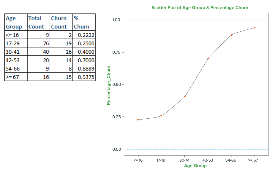
The above scatterplot illustrates that the relationship between AgeGroup and Churn resembles like a S-shaped curve. Here, we have only 6 Age Groups for this data resulting into – a look like S-curve. But with the addition of more data resulting into many Age Groups, we would get a clear smooth S-curve. The S-curve does a better job of “fitting” these data points rather than the best fit straight line (obtained by Linear Regression).
Now, the question arises – whether this fitted curve results in prediction of Churn values as finite (‘0’ or ‘1’)?
To answer this question, let’s assume a cut-off point say 0.5 to differentiate the user’s behavior and estimate the chance of the user’s churn tendency. Now let’s define the rule to achieve this –
This rule enables us to get the response values only as either ‘0’ or ‘1’, which is in sync with the nature of Churn variable.
But, this method is difficult in practice, as the determination of ideal cut-off point to arrive at AgeGroups is tedious and time-consuming. Hence, we need to resort to use some methodology to cater to these issues of the data easily.
Now, in view of the Churn-Age dataset, let’s define some more terms that are frequently encountered, discuss how these terms are related to one another and how they are useful for logistic regression.
Probability – is the quantitative representation of the chance that an event will occur. For instance, let’s define an event as “retaining the user for a particular AgeGroup” – that is, obtain the desired outcome value as “1” – which signifies “No Churn”. Thus, the Churn Percentage that we computed above, is actually the chance (probability) that we get a success as per the above defined event.
In short, probability is the number of times the events “occurs” divided by the total number of times the event “could occur”.
Odds – is always in relation to the happening of an event. We often use terms like – What is the odds that “It will rain today” or “Team A will win”. Odds is defined as the ratio of the chance of the event happening to that of non-happening of the event.
For instance, with our Churn-Age example, for an AgeGroup – “42-53” years, the probability of an event – User not churning is 14/20 = 0.7 and the probability of an event – User churning out is (1-0.7) = 0.3. Hence the odds of user churning out for individuals falling under “42-53” years is 0.7 / 0.3 = 2.33. That implies, the chance of user belonging to “42-53” years will not churn is little over than twice the chance that the user will churn out.
Note that odds can be converted back into probability as
$ Odds = \frac{Probability \ of \ Success}{Probability \ of \ Failure} = \frac{p}{1 – p} \textit{ OR } $
$ Probability = \frac{odds}{1 + odds} $
In common sense, probability and odds are used interchangeably. However, in statistics, probability and odds are not the same, but different.
The dataset (with these relevant terms) is displayed below, which forms the basis for building Logistic Regression model.
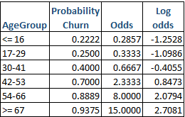
As in the above table, we have moved from Probability to Odds to Log of odds. But why do we need to take all the trouble to do the transformation to Log odds?
Probability ranges from 0 to 1 whereas Odds range from 0 to +ꝏ. The odds increase as the probability increases or vice versa, i.e. for higher probabilities, say p = 0.9, 0.999, 0.9999, Odds will be 9, 999, 9999 respectively.
Usually, it is difficult to model a variable which has restricted range, such as probability as it bounds between 0 and 1. Hence, we model odds of a variable to get around the restricted range problem.
But why Log transformation? There are two reasons for selecting “Log” as below:
How to build a logistic regression model with Log odds?
Let ‘y’ be the outcome variable (say User Churn) indicating failure / success with 0 / 1 and ‘p’ be the probability of y to be 1 i.e. p = Prob (y=1). Let x1, x2,…., xk be a set of predictor variables (say, User Age, Gender and so on).
Then, the logistic regression model equation of y given x1, say User Churn given Age, can be written as below:
$ log\left ( odds \right ) = log\left (\frac{p}{1 – p} \right ) = \left (a + b_{1}x_{1} \right ) $
The above model equation expresses the log-odds of an event as a linear function of its predictors.
But we need the outcome value as either 0 or 1 i.e. we need back the probabilities as outcome value. This can be obtained by taking an exponent of the above equation as shown below:
$ exp\left ( log\left (\frac{p}{1 – p} \right ) \right ) = exp\left ( a + b_{1}x_{1}\right )$
$ \Rightarrow \frac{p}{1 – p} = exp\left (a + b_{1}x_{1}\right ) { [Since \ exp (log x) = x]} $
Solving the above equation for p, we get
$ p = \frac{exp\left (a + b_{1}x_{1} \right )}{1 + exp\left (a + b_{1}x_{1} \right )}$
The above function of ‘p’ is known as “Sigmoidal” function and its plot (S-shaped curve) is as below: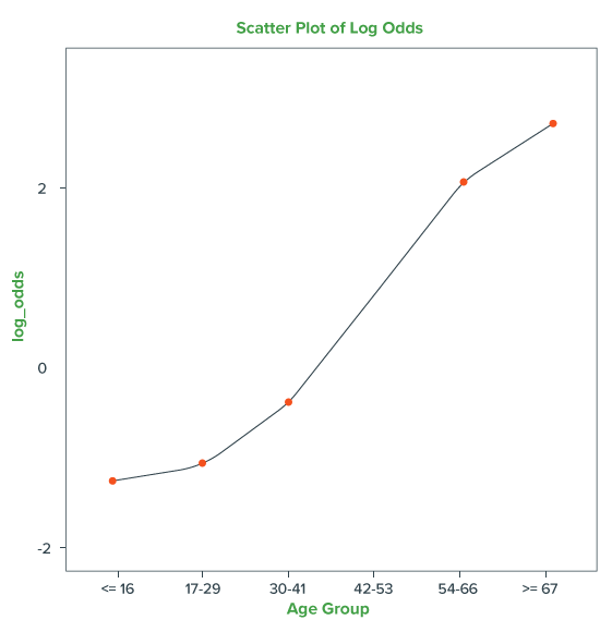
Thus, with this simple example of User Churn-Age dataset, we could decipher the intuition behind the Math of Logistic Regression.
Closing Thoughts
Logistic Regression is simply an extension of the linear regression model, so the basic idea of prediction is the same as that of Multiple Regression Analysis. But, unlike the multiple regression model, the logistic regression model is designed to test response variables, having finite outcomes.
Although logistic regression does contain a few complexities and new statistical concepts, it is within reach of anyone who can use linear models. Similar to Linear Regression, Logistic regression model provides the conceptual foundation for more sophisticated statistical and machine learning approaches.
In the next part, we will delve deeper into the Assumptions, Model Interpretation and Evaluation of Logistic Regression Model.
Source code to reproduce the examples mentioned in this article is available here. Read another one of our popular article, The Fallacy of Patterns here.